Credibility Analysis for Mortality Experience Studies, Part 1
March  2008

​​​​​​The bane of pricing actuaries is their desire for more and more data in a preferred risk environment that is designed to produce fewer and fewer deaths. Previous mortality experience can be a reliable indicator of the future performance as long as one understands the potential variability in these future results. To that end, I would like to discuss the theory that actuaries often use to analyze the credibility of their mortality studies.

Mortality as a Binomial Process
Consider a random experiment, the outcome of which can be classified in only one of two mutually exclusive ways. Since we are applying this theory to mortality, we will use the morbidly descriptive titles “dead” or “alive.” We have the following conditions:

• Assume that we have n independent trials, and we count the number of deaths over some time period. For a mortality study, each trial represents a risk with the probability of either dying or living during a specified time period, which is typically one calendar year.
• Let the probability of dying = q, and the probability of living = p. Note that q + p = 1.
• Let the random variables X₁, X₂, X₃, ... X_n be mutually exclusive stochastic (i.e., random) events where Xi equals 1 if death occurred and 0 if no death occurred.

If the above conditions are met, then the random variable Y, which we set equal to the sum of the X’s, has what statisticians call a binomial distribution. Because of the way we assigned values to the X’s, Y equals the number of deaths that occur among our n risks. In mathematical terms, the probability that our random variable Y equals a specific value y can be written as:

Pr (Y = y) = (“n choose y”) * q^y * p^(n-y)

Plainly speaking, this means: take all the possible ways you can choose y risks out of a group of n risks and multiply that by the probabilities that (i) all of the y risks die and (ii) all of the remaining (n-y) live.

The number of claims is binomially distributed with a mean value of (n * q). More importantly, the binomial has an easily calculated variance of (n * q * p).

The standard deviation, which is the square root of the variance, is a measure of the inherent variability of the outcome of our mortality “experiment” and provides the basis for discussions on credibility.

An Example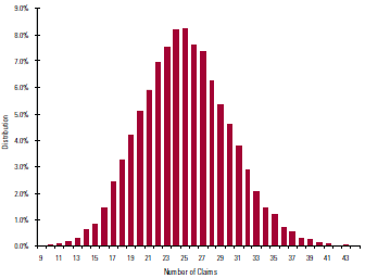

Before we go any further, a sample experiment may help demonstrate these concepts. Consider the following parameters:

• 20,000 risks (n)
• Probability of death is 0.00125 (q)
• Probability of living is 0.99875 (p)
• The theoretical mean of the distribution is 25 (n * q)
• The theoretical standard deviation of the distribution is 5 (square root of [n * p * q])

Chart 1 above shows the results of 10,000 independent experiments on these 20,000 risks by graphing the resulting claim count distribution.

With 10,000 experiments, our sample statistics should closely match theoretical values. In fact, the mean number of claims from our 10,000 experiments is 25.02 and the standard deviation is 4.96, which tie to the theoretical mean 25 and standard deviation of 5.

Standard Deviation as a Measure of Credibility
We can create a “credibility measure” to help understand the variability of these results by taking the ratio of the standard deviation over the mean.

A highly credible experiment would be where the range of outcomes as a percentage of the mean is very low. In other words, the distribution of the number of deaths is tightly packed around the sample mean.

For our current example, the number of deaths as a percentage of the mean varies quite a bit. Approximately 70 percent of our results are inside plus or minus 20 percent (i.e., inside the range of 20 to 30 claims). Thus, if I were to predict the number of deaths in a given random sample within a range of plus or minus 20 percent, I would be wrong 30 percent of the time.

Our credibility measure is mathematically equivalent to the square root of (p / # deaths), which can be simplified further to (1 / square root of # deaths) because p for mortality studies is typically close to 1. Chart 2 shows our credibility measure for different size experiments using the same probability of death as our current example.

Chart 2 - Credibility Measure for Various Size Experiments

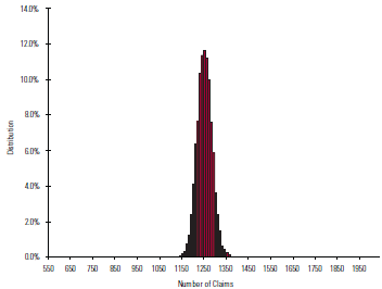
So, if the number of risks in our experiment was 1,000,000, and I were to make an advance guess of the results of one particular random sample within a range of only plus or minus 2.8 percent of the mean, I would be wrong 30 percent of the time.

However, a better way to describe this might be to say that my guess within a range of plus or minus 20 percent of the mean would be correct more than 99.99999 percent of the time. Thus, as the number of deaths increases, I can be more confident in my prediction of the results of any one particular random sample. Chart 3 graphically demonstrates this statement.

Relationship to Mortality Studies
This article has explained some of the basic tools that actuaries use to project variability around predicted mortality. Simply stated, a mortality study is nothing more than the result of one random sample from a large universe of possible outcomes. The actuary’s job is to describe how well that one sample represents the universe and to what degree that sample’s results can be used to predict future outcomes.

In Part 2 of this series I build upon these fundamental concepts by discussing what exactly is meant by the term “fully credible” when applied to mortality studies.